The concept of ‘mean reversion’ is part of both, our everyday life as well as investing. However, inadequate understanding of the ‘mean’ leads to several mistakes in the application of this concept. When it comes to equities, over the long run share prices revert to their fundamentals and hence, clarity of thought around fundamental strengths of a business and its longevity becomes very important in equity investments.
Performance update – as on 30th June 2020
We have coverage universe of around 25 stocks, which have historically delivered a high degree of consistency in ROCE and revenue growth rates. Our research team of nine analysts focuses on understanding the reasons why companies in our coverage universe have consistently delivered superior financial performance. Based on this understanding, we construct a concentrated portfolio of companies with an intended average holding period of stocks of 8-10 years or longer. The latest performance of our PMS and offshore fund (USD denominated) portfolios is shown in the charts below.
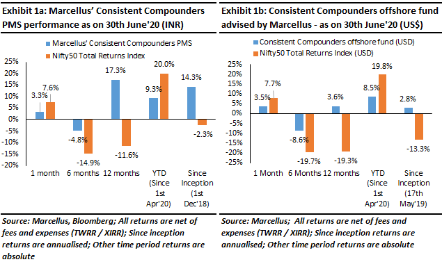
Although we have outperformed against Nifty50 over the past six months and longer time periods, our underperformance over the past 1 month and 3 months against Nifty50 is driven by three broad factors. Firstly, our portfolio’s outperformance over a longer term is likely to closely track the differential in earnings growth rates for our portfolio vs Nifty50. Whilst this differential in earnings growth has historically been around 10%-15%, our portfolio’s outperformance on a 12-month basis had increased to ~33% as on 31st March 2020. Secondly, a mathematical illusion in short term alpha kicks in when stock prices become highly volatile. An example to extrapolate this illusion – if over 3 months, Stock A falls by 80% and Stock B falls by 50%, the alpha of Stock B over Stock A is +30%. In the subsequent 3 months, if Stock A rises by 100% and Stock B rises by 50%, the alpha of Stock B over Stock A during these three months is -50%. However, for the overall six months period, Stock B outperformed over Stock A by +35% (rather than the optical illusion of adding up +30% and -50% and concluding that Stock B might not have outperformed over Stock A meaningfully during the six month period). When it comes to Marcellus’ CCP, almost half of the 3-month underperformance can be attributed to this optical illusion. And thirdly, Reliance Industries has single handedly contributed 6% to the overall performance of Nifty50 over the past three months. We do not have Reliance Industries in our coverage universe (and hence in our clients’ portfolios).
Concept of ‘mean reversion’ – the risk of applying it in investing without understanding it adequately!
The basic definition of ‘mean reversion’ is that asset prices and historical returns will revert to the long-run mean or average level of the entire dataset. The concept hopes to identify abnormal activity that will revert to a normal pattern in future. In other words, ‘mean reversion’ suggests that cumulative observations matter more than the most recent one.
Many of you would have come across the following statements related to ‘mean reversion’ while investing in equities:
Booking profits (vs booking losses):
“Since I have to sell part of my equity portfolio, let me sell stock A where I am making a profit rather than selling Stock B where I will have to book a loss.”
Investing at 52 week high!:
“I want to add two stocks to my portfolio – Stock A and Stock B. Stock A is trading close to its 52 week high while Stock B is trading close to its 52 week low. Hence, I should buy Stock B now and I should wait for Stock A to fall before I decide to buy it.”
Investing at rich P/E multiples:
“Current P/E multiple of Stock A is 30% higher than its average P/E multiple for the last 10 years. Hence, Stock A is expensive.”
Often, the concept of mean reversion fails to hold true for these three statements. Why?
In our everyday life, we clearly demarcate between areas where ‘mean reversion’ applies and areas where it does not apply. For example, if the city of Mumbai receives rainfall on a day in the month of January, we do not see shoppers on the high-street buying several umbrellas and raincoats. This is because the concept of mean reversion holds true and shoppers do not expect unseasonal rainfall to continue over the next few days. Our cumulative observations over many years matter more than the most recent observation.
Here is another example. A father has two children – a son and a daughter. The daughter always ranks amongst the top 10% of all students in her school (like a stock trading at its 52-week high). The son always ranks amongst the bottom 10% of all students in his school (like a stock’s 52-week low). The mean (average) performance between the two children is around the fifth decile. While planning for his children’s future, this father does not expect ‘mean reversion’ to result in his daughter’s performance to drop down to the fifth decile in future. Why? Because the father understands the factors that have driven the daughter’s strong performance and hence if these driving factors sustain into the future, then her strong performance will also continue in future. In other words, the father understands that the real ‘mean’ applicable for his daughter is the historical track record of top decile performance, and not the fifth decile which is the average of the two children.
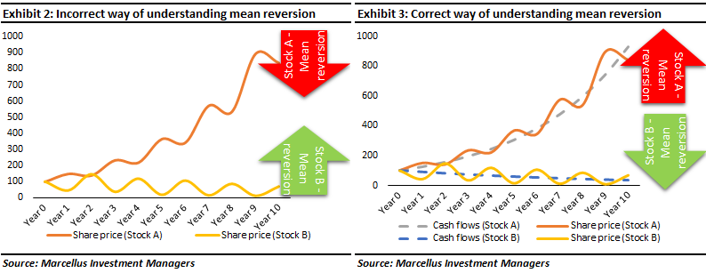
The key to understanding how and where mean reversion applies, lies in the correct understanding of the ‘mean’ itself. For instance, in the exhibit on the left below, incorrect understanding of the underlying fundamentals (i.e. the ‘mean’) leads to incorrect decision making by the investor, an error which can only be avoided by correct understanding of ‘mean’ – as shown in the exhibit on the right below
|
||||

